This analysis focuses on the proportion of serious crimes (“felony assault”) and aims to investigate the socioeconomic factors associated with the higher rate of serious crimes. Again, we used 2021 NYPD crime complaint data and 2020 Census population data.
The primary outcome (dependent variable: fel_asslt_rate) is the number of felony assault cases in each precinct divided by the total number of complaints in each precinct.
NYC Open Data (2013) was used as spatial data to determine the borders of each precinct.

# import and clean NYPD data
df_nypd = read_csv("https://www.dropbox.com/scl/fi/kf2zk4t1onxzm2vo3lpkq/NYPD_Complaint_Data_Historic.csv?rlkey=ly36vi9v66sno80eir6rohlwn&dl=1", na = "(null)") |> # some values are coded as "(null)" in the df; rewrite them as NA
  janitor::clean_names()

# precinct neighbor association
prec_neighbor = read_csv("data/nyc_prec_neighborhood.csv")


# merging neighborhood information with NYPD data, keep only relevant variables
nypd_ses_df = df_nypd |> 
  rename(precinct = addr_pct_cd) |> 
  mutate(cmplnt_fr_dt = as.Date(cmplnt_fr_dt, format = "%m/%d/%Y"),
         year = format(cmplnt_fr_dt, "%Y")) |> 
  left_join(prec_neighbor, by = "precinct") |> 
  filter(year == 2021) |> 
  select(precinct, ofns_desc, neighborhood, borough, longitude, latitude) |> 
  drop_na()

#Import and clean socio-economic data. neighbor_SES has SES indicators (except rent) for each neighborhood 
neighbor_ses = readxl::read_excel("data/neighorhood_indicators.xlsx", sheet = "Data") |> 
  janitor::clean_names() |> 
  filter(region_type == "Sub-Borough Area") |> 
  rename(neighborhood = region_name) |> 
  select(neighborhood, year, hh_inc_med_adj, pop16_unemp_pct, pop_edu_collp_pct, pop_pov_pct, pop_race_asian_pct, pop_race_black_pct, pop_race_hisp_pct, pop_race_white_pct, pop_foreign_pct) |> 
  filter(year == 2021) |> 
  mutate(
    pop16_unemp_pct = pop16_unemp_pct * 100, 
    pop_edu_collp_pct = pop_edu_collp_pct * 100, 
    pop_pov_pct = pop_pov_pct * 100,
    pop_race_asian_pct = pop_race_asian_pct * 100, 
    pop_race_black_pct = pop_race_black_pct * 100, 
    pop_race_white_pct = pop_race_white_pct * 100, 
    pop_race_hisp_pct = pop_race_hisp_pct * 100, 
    pop_foreign_pct = pop_foreign_pct * 100
  ) 

# NYC neighborhoods borders
nyc = read_sf(here::here("data", "Police_Precincts.geojson")) |> 
  select(-shape_area, -shape_leng) |> 
  mutate(
    precinct = as.double(precinct)
  )

# population data by precinct (2020 census, P1_001N: total population)
df_pop = read_csv(here::here("data", "nyc_precinct_2020pop.csv")) |> 
  rename(pop = P1_001N) |> 
  select(precinct, pop)

# merge with nypd dataset and calculate relevant indicators
nypd_ses_sda = nypd_ses_df |>  
  left_join(neighbor_ses, by = "neighborhood") |> # combine with ses data
  st_as_sf(
    # which columns to use as coordinates
    coords = c("longitude", "latitude"), 
    # keep the coordinate columns
    remove = FALSE,
    # projection system
    crs = 4326
  ) |> 
  merge(df_pop, by = "precinct") |> 
  group_by(precinct) |> 
  mutate(
    "fel_asslt_rate" = (sum(ofns_desc == "FELONY ASSAULT") / n()) * 100 # calculate "FELONY ASSAULT" rate among all crimes 
  ) |> 
  select(precinct, neighborhood, borough, pop, hh_inc_med_adj, pop16_unemp_pct, pop_edu_collp_pct, pop_pov_pct, geometry, fel_asslt_rate, pop_race_asian_pct, pop_race_black_pct, pop_race_white_pct, pop_race_hisp_pct, pop_foreign_pct) |> 
  ungroup()

# spatial join
df_spj = nypd_ses_sda |>
  # spatial join
  st_join(
    # only need these columns from nyc tibble
    nyc |> select(precinct, geometry),
    # join rows where there is some overlap between a dock and a precinct
    join = st_intersects,
    left = FALSE
  ) |> 
  select(-precinct.y) |> 
  rename(precinct = precinct.x)

count_by_precinct = df_spj |> 
  # remove geometry for fast counting
  st_drop_geometry() |> 
  distinct() |> 
  # join the counts into the nyc neighborhood object
  right_join(nyc, by=c("precinct" = "precinct")) |> 
  mutate(
    "pre_nei" = paste(precinct, "-", neighborhood, sep = " ") 
  ) |> 
  st_as_sf() |> 
  filter(precinct != 22) # remove central park data

We built the following three models and compered their performance.
- Standard linear regression
- Spatial lag model (SLM)
- Spatial error model (SEM)

# simple linear regression
fit.ols.simple = lm(fel_asslt_rate ~ hh_inc_med_adj, data = count_by_precinct)

# multiple linear regression
fit.ols.multiple = lm(fel_asslt_rate ~ log(pop) + hh_inc_med_adj + pop16_unemp_pct + pop_edu_collp_pct + pop_pov_pct + pop_race_asian_pct + pop_race_black_pct + pop_race_white_pct + pop_race_hisp_pct + pop_foreign_pct, data = count_by_precinct)

# the neighbor nb object using poly2nb()
seab = poly2nb(count_by_precinct, queen = T)

# the listw weights object using nb2listw()
seaw = nb2listw(seab, style = "W", zero.policy = TRUE)

# Spatial lag model (SLM)
fit.lag = lagsarlm(fel_asslt_rate ~ log(pop) + hh_inc_med_adj + pop16_unemp_pct + pop_edu_collp_pct + pop_pov_pct + pop_race_asian_pct + pop_race_black_pct + pop_race_white_pct + pop_race_hisp_pct + pop_foreign_pct, data = count_by_precinct, listw = seaw) 

# get estimates of the direct, indirect and total effect of each variable
fit.lag.effects = impacts(fit.lag, listw = seaw, R = 999)

# Spatial error model (SEM)
fit.err = errorsarlm(fel_asslt_rate ~ log(pop) + hh_inc_med_adj + pop16_unemp_pct + pop_edu_collp_pct + pop_pov_pct + pop_race_asian_pct + pop_race_black_pct + pop_race_white_pct + pop_race_hisp_pct + pop_foreign_pct, data = count_by_precinct, listw = seaw)

First, let’s look at the histogram of the dependent variable. The distribution is unimodal and slightly right-skewed, but overall it is approximately normally distributed.

# histogram
count_by_precinct |> 
  ggplot() +
    geom_histogram(aes(x = fel_asslt_rate)) +
    xlab("Felony assault rate")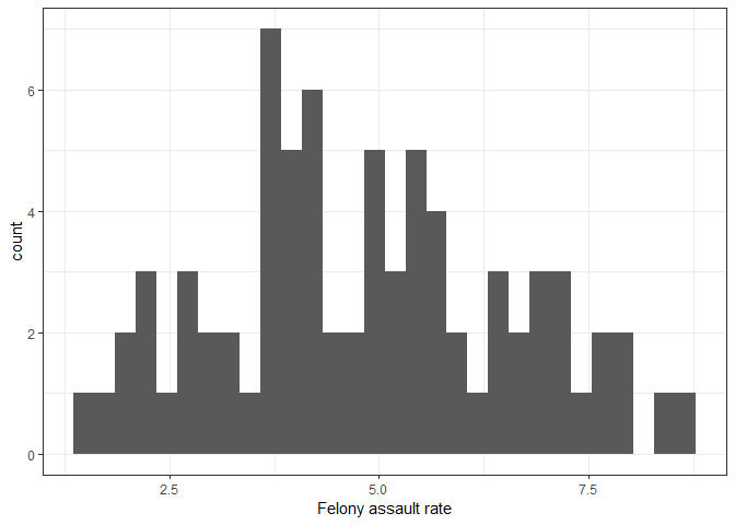

Explaratory spatial data analysis

# ESDA
tmap_mode("plot")

tm_shape(count_by_precinct, unit = "mi") +
  tm_polygons(col = "fel_asslt_rate", style = "quantile", palette = "Reds", title = "") +
  tm_scale_bar(breaks = c(0, 2, 4), text.size = 1, position = c("right", "bottom")) +
  tm_layout(main.title = "Felony assault rate, 2021",  main.title.size = 0.95, frame = FALSE, legend.outside = TRUE, 
            attr.outside = TRUE)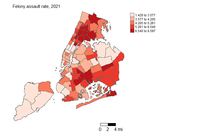

# plot residuals
count_by_precinct = count_by_precinct |> 
  mutate(olsresid = resid(fit.ols.multiple))

tm_shape(count_by_precinct, unit = "mi") +
  tm_polygons(col = "olsresid", style = "quantile",palette = "Reds", title = "") +
  tm_scale_bar(breaks = c(0, 2, 4), text.size = 1, position = c("right", "bottom")) +
  tm_layout(main.title = "Residuals from linear regression",  main.title.size = 0.95, frame = FALSE, legend.outside = TRUE,
            attr.outside = TRUE)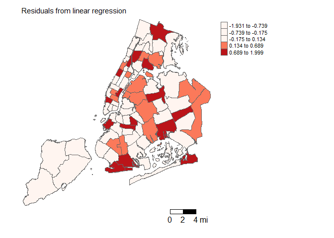

The spatial distribution of precincts with high felony crime rates and the residuals of the linear regression model are visualized. Spatial autocorrelation of errors is indicated as both maps appear to cluster.

# examine the Moran scatterplot
moran.plot(as.numeric(scale(count_by_precinct$fel_asslt_rate)), listw = seaw, 
           xlab = "Standardized Felony Assault Rate", 
           ylab = "Precincts Standardized Felony Assault Rate",
           main = c("Moran Scatterplot for Felony assault rate in NYC"))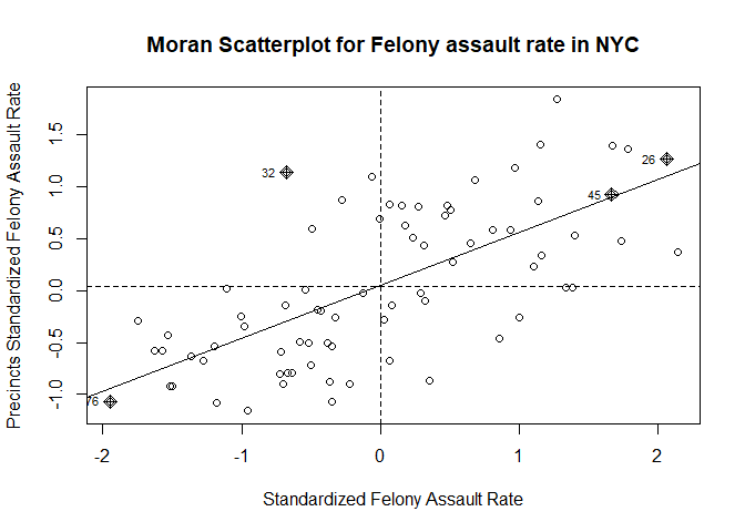

The Moran scatter plot displays the positive relationship between the standardized felony assault rate and precincts standardized felony assault rate.

# the Global Moran’s I
# use Monte Carlo simulation to get the p-value
moran.mc(count_by_precinct$fel_asslt_rate, seaw, nsim=999) |> 
  broom::tidy() |> 
  knitr::kable()

statistic	p.value	parameter	method	alternative
0.5097451	0.001	1000	Monte-Carlo simulation of Moran I	greater

# repeat for the OLS residuals using the lm.morantest() function
lm.morantest(fit.ols.multiple, seaw) |> 
  broom::tidy() |> 
  knitr::kable()

estimate1	estimate2	estimate3	statistic	p.value	method	alternative
-0.115526	-0.082871	0.0056489	-0.4344796	0.6680299	Global Moran I for regression residuals	greater

The Moran I test indicates that there is a positive spatial autocorrelation for the felony assault rate, but no spatial autocorrelation for the linear regression residuals.

Compare three models

# present results for more than one model
stargazer(fit.ols.multiple, fit.lag, fit.err, type = "html", digits = 3, title = "Regression Results")

**Regression Results**

	Dependent variable:

	fel_asslt_rate
	OLS	spatial	spatial
		autoregressive	error
	(1)	(2)	(3)

log(pop)	-0.150	-0.150	-0.192
	(0.336)	(0.310)	(0.283)

hh_inc_med_adj	0.00001	0.00001	0.00001
	(0.00001)	(0.00001)	(0.00001)

pop16_unemp_pct	-0.007	-0.002	-0.006
	(0.059)	(0.055)	(0.049)

pop_edu_collp_pct	0.0005	0.001	0.002
	(0.015)	(0.013)	(0.011)

pop_pov_pct	0.089^**	0.090^***	0.099^***
	(0.036)	(0.033)	(0.028)

pop_race_asian_pct	-0.102^*	-0.107^**	-0.108^**
	(0.055)	(0.052)	(0.044)

pop_race_black_pct	-0.033	-0.036	-0.044
	(0.056)	(0.052)	(0.045)

pop_race_white_pct	-0.078	-0.082^*	-0.091^**
	(0.052)	(0.048)	(0.042)

pop_race_hisp_pct	-0.053	-0.056	-0.063
	(0.050)	(0.046)	(0.040)

pop_foreign_pct	0.031^*	0.031^*	0.033^**
	(0.017)	(0.016)	(0.014)

Constant	9.499	10.060^*	10.531^*
	(6.510)	(6.077)	(5.414)


Observations	76	76	76
R²	0.761
Adjusted R²	0.724
Log Likelihood		-95.441	-93.988
sigma²		0.721	0.674
Akaike Inf. Crit.		216.882	213.976
Residual Std. Error	0.920 (df = 65)
F Statistic	20.697^*** (df = 10; 65)
Wald Test (df = 1)		0.287	4.691^**
LR Test (df = 1)		0.250	3.156^*

Note:	p<0.1; p<0.05; p<0.01

# save AIC values
AICs = c(AIC(fit.ols.multiple),AIC(fit.lag), AIC(fit.err))
labels = c("Standard Linear Regression", "Spatial Lag Model","Spatial Error Model" )

data.frame(Models = labels, AIC = round(AICs, 2)) |> 
  knitr::kable()

Models	AIC
Standard Linear Regression	215.13
Spatial Lag Model	216.88
Spatial Error Model	213.98

The Akaike Information Criterion (AIC) values across the three models suggest that the spatial error model (SEM) is the best fit of the three models.

The coefficients of pop_pov_pct, pop_race_asian_pct, pop_race_white_pct and pop_foreign_pct were statistically significant in the spatial error model.

Linear regression diagnostics

# diagnostics
ggplot() + 
  geom_histogram(mapping = aes(x=resid(fit.ols.multiple))) +
  xlab("OLS residuals")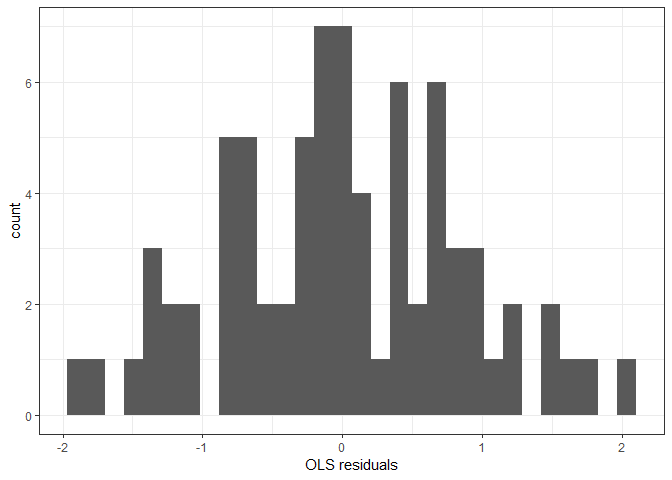

qqPlot(fit.ols.multiple)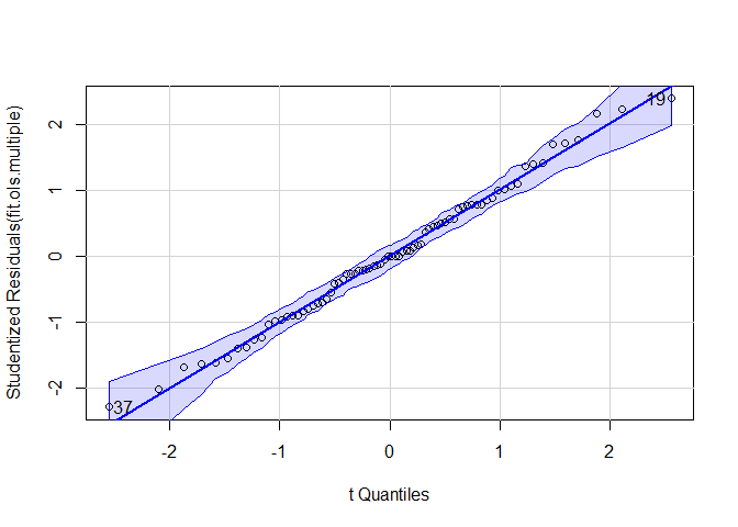

## [1] 19 37

plot(resid(fit.ols.multiple))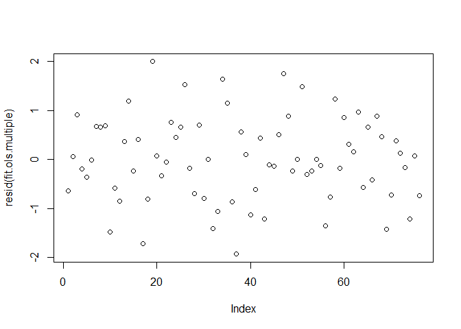

OLS residuals are normally distributed and Q-Q plot also indicates that the normality assumption is met in this model. There may be heteroskedasticity according to the third plot, where the points are narrowing as the index moves from left to right.

Conclusion

The spatial error model demonstrated a superior fit, revealing that factors such as the poverty rate, the percentage of Asian and White populations, and the percentage of individuals born outside the US or Puerto Rico were significant predictors for serious crime rates.

References

NYPD (2023, June 16). NYPD Complaint Data Historic: NYC Open Data. Link
CoreData.nyc. Subsidized Housing Database. NYU Furman Center’s CoreData.nyc. Link
Bureau, U. C. (2022, November 29). 2020 census. Census.gov. Link
Department of City Planning (DCP) (2013, Jan 29). NYC Open Data. Link

Factors associated with serious crimes

Explaratory spatial data analysis

Compare three models

Linear regression diagnostics

Conclusion

References