Exploratory Data Visualization
While examining the NYPD crime complaint data, we expect crime rate
to be indicative by the socioeconomic status of a specific neighborhood.
In this section, we calculated the crime rate for each neighborhood each
year, visualized various socioeconomic status by each police precint
(neighborhood), and displayed the top neighborhoods with highest crime
rate, along with what their crime composition looks like. We are also
interested in whether crime rate can be predictive of rent in
corresponding neighborhoods.
Since the primary data used did not have neighborhood information, we
used NYPD precinct data to classify neighborhoods, following Golub et
al. (2006)
# Import and clead NYPD data
df_nypd = read_csv("https://www.dropbox.com/scl/fi/kf2zk4t1onxzm2vo3lpkq/NYPD_Complaint_Data_Historic.csv?rlkey=ly36vi9v66sno80eir6rohlwn&dl=1", na = "(null)") |> # some values are coded as "(null)" in the df; rewrite them as NA
janitor::clean_names()
prec_neighbor = read_csv("data/nyc_prec_neighborhood.csv")
#Merging neighborhood information with NYPD data, keep only relevant variables
nypd_ses_df = df_nypd |>
select(cmplnt_num, cmplnt_fr_dt, addr_pct_cd, crm_atpt_cptd_cd, law_cat_cd, susp_age_group, susp_race, susp_sex, vic_age_group, vic_race, vic_sex, ofns_desc, pd_desc, latitude, longitude) |>
rename(precinct = addr_pct_cd) |>
mutate(cmplnt_fr_dt = as.Date(cmplnt_fr_dt, format = "%m/%d/%Y"),
year = format(cmplnt_fr_dt, "%Y")) |>
left_join(prec_neighbor, by = "precinct")
#Import and clean socio-economic data. neighbor_SES has SES indicators (except rent) for each neighborhood
neighbor_ses = readxl::read_excel("data/neighorhood_indicators.xlsx", sheet = "Data") |>
janitor::clean_names() |>
filter(region_type == "Sub-Borough Area") |>
rename(neighborhood = region_name) |>
select(neighborhood, year, pop_num, hh_inc_med_adj, pop16_unemp_pct, pop_edu_collp_pct, pop_edu_nohs_pct, pop_pov_pct, pop_race_asian_pct, pop_race_black_pct, pop_race_hisp_pct, pop_race_white_pct, pop_foreign_pct) |>
filter(year %in% c(2017, 2018, 2019, 2020, 2021, 2022))
#neighbor_rent has rent data for each neighborhood
neighbor_rent = readxl::read_excel("data/neighorhood_indicators.xlsx", sheet = "Data") |>
janitor::clean_names() |>
filter(region_type == "Sub-Borough Area") |>
rename(neighborhood = region_name) |>
filter(year == "2017-2021") |>
select(neighborhood, gross_rent_0_1beds, gross_rent_2_3beds)
#ses_df has crime rate and SES indicators for each neighborhood
ses_df = nypd_ses_df |>
group_by(year, borough, neighborhood) |>
summarise(crime_num = n())
ses_df = ses_df |> merge(neighbor_ses, by = c("year", "neighborhood")) |>
mutate(crime_rate = (crime_num/pop_num) * 100,000) |>
left_join(neighbor_rent, by = "neighborhood")Cloropleth maps
Data
In this section, we mapped the crime rate (with a specific focused on
“felony assault”) and the socioeconomic status in each police precinct.
The data used for this analysis were 2021 NYPD crime complaint data and
2020 Census population data.
Crimes categorized under “felony assault” share common characteristics
such as physical injury, intentional and reckless actions, the use of
deadly weapons or dangerous instruments, and others as defined by New
York Penal Law.
The serious crime rate was determined by dividing the total number of
felony assault complaints in each precinct by the total population in
that precinct. Note that due to lack of data, data on crime complaints
and socioeconomic status are based on 2021 records, while data on total
population are from 2020.
# NYC neighborhoods borders
nyc = read_sf(here::here("data", "Police_Precincts.geojson")) |>
select(-shape_area, -shape_leng) |>
mutate(
precinct = as.double(precinct)
)
# prepare data set for mapping
# population data by precinct (2020 census, P1_001N: total population)
df_pop = read_csv(here::here("data", "nyc_precinct_2020pop.csv")) |>
rename(pop = P1_001N) |>
select(precinct, pop)
# select ses variables
ses_heat = neighbor_ses |>
filter(year == 2021) |> # visualize 2021 data
mutate(
pop16_unemp_pct = pop16_unemp_pct * 100,
pop_edu_collp_pct = pop_edu_collp_pct * 100,
pop_pov_pct = pop_pov_pct * 100
) |>
select(neighborhood, pop_num, hh_inc_med_adj, pop16_unemp_pct, pop_edu_collp_pct, pop_pov_pct)
# merge with nypd dataset and calculate relevant indicators
nypd_ses_heat = nypd_ses_df |>
filter(year == 2021) |>
left_join(ses_heat, by = "neighborhood") |> # combine with ses data
st_as_sf(
# which columns to use as coordinates
coords = c("longitude", "latitude"),
# keep the coordinate columns
remove = FALSE,
# projection system
crs = 4326
) |>
merge(df_pop, by = "precinct") |>
group_by(precinct) |>
mutate(
"s_crime_rate" = (sum(ofns_desc == "FELONY ASSAULT") / pop) * 100000, # calculate crime rate per 100,000 using 2020 population census data by precinct
"violation" = (sum(law_cat_cd == "VIOLATION") / n()) * 100, # the rate of violation among all complaints
"misdemeanor" = (sum(law_cat_cd == "MISDEMEANOR") / n()) * 100, # the rate of misdemeanor among all complaints
"felony" = (sum(law_cat_cd == "FELONY") / n()) * 100 # the rate of felony among all complaints
) |>
select(precinct, neighborhood, hh_inc_med_adj, pop16_unemp_pct, pop_edu_collp_pct, pop_pov_pct, geometry, s_crime_rate, felony, misdemeanor, violation)
# spatial join
df_spj = nypd_ses_heat |>
# spatial join
st_join(
# only need these columns from nyc tibble
nyc |> select(precinct, geometry),
# join rows where there is some overlap between a dock and a precinct
join = st_intersects,
left = FALSE
) |>
select(-precinct.y) |>
rename(precinct = precinct.x)
count_by_neighborhood = df_spj |>
# remove geometry for fast counting
st_drop_geometry() |>
distinct() |>
# join the counts into the nyc neighborhood object
right_join(nyc, by=c("precinct" = "precinct")) |>
mutate(
"pre_nei" = paste(precinct, "-", neighborhood, sep = " ")
) |>
st_as_sf() |>
filter(precinct != 22) # remove central park dataLevel of offense
This map shows the proportion of different offense levels among all complaints reported in each precinct/neighborhood.
# tmap
tmap_mode("view") # set tmap to the view mode
tm_shape(count_by_neighborhood) +
tm_polygons(col = c("violation", "misdemeanor", "felony"), id = "pre_nei", title = c("Violation (%)", "Misdemeanor (%)", "Felony (%)"), popup.vars = c("Violation: " = "violation", "Misdemeanor: " = "misdemeanor", "Felony: " = "felony")) +
tm_facets(sync = TRUE, ncol = 3)Median household’s income
The median household’s total income of all members of the household aged 15 years or older.
tm_shape(count_by_neighborhood) +
tm_polygons(col = "hh_inc_med_adj", id = "pre_nei", title = "Median income (USD/yr)", palette = "Blues", popup.vars = c("Median houshold's income: " = "hh_inc_med_adj", "Serious crime rate (per 100,000): " = "s_crime_rate")) +
tm_bubbles("s_crime_rate", id = "pre_nei", col = "azure", alpha = .5, popup.vars = c("Median houshold's income: " = "hh_inc_med_adj", "Serious crime rate (per 100,000): " = "s_crime_rate"))Unemployment rate
The number of people aged 16 years and older in the civilian labor force who are unemployed, divided by the total number of people aged 16 years and older in the civilian labor force.
tm_shape(count_by_neighborhood) +
tm_polygons(col = "pop16_unemp_pct", id = "pre_nei", title = "Unemployment rate (%)", popup.vars = c("Unemployment rate: " = "pop16_unemp_pct", "Serious crime rate (per 100,000): " = "s_crime_rate")) +
tm_bubbles("s_crime_rate", id = "pre_nei", col = "azure", alpha = .5, popup.vars = c("Unemployment rate: " = "pop16_unemp_pct", "Serious crime rate (per 100,000): " = "s_crime_rate"))Education
The percentage of the population aged 25 and older who have attained a bachelor’s degree or higher.
tm_shape(count_by_neighborhood) +
tm_polygons(col = "pop_edu_collp_pct", id = "pre_nei", title = "College graduates (%)", palette = "Blues", popup.vars = c("College graduates: " = "pop_edu_collp_pct", "Serious crime rate (per 100,000): " = "s_crime_rate")) +
tm_bubbles("s_crime_rate", id = "pre_nei", col = "azure", alpha = .5, popup.vars = c("College graduates: " = "pop_edu_collp_pct", "Serious crime rate (per 100,000): " = "s_crime_rate"))Poverty
The number of people below the poverty threshold divided by the number of people for whom poverty status was determined. The poverty threshold in 2021 was $27,479 for a family of four (two adults and two children under 18 years).
tm_shape(count_by_neighborhood) +
tm_polygons(col = "pop_pov_pct", id = "pre_nei", title = "Below poverty threshold (%)", popup.vars = c("Below poverty threshold: " = "pop_pov_pct", "Crime rate (per 100,000): " = "s_crime_rate")) +
tm_bubbles("s_crime_rate", id = "pre_nei", col = "azure", alpha = .5, popup.vars = c("Below poverty threshold: " = "pop_pov_pct", "Serious crime rate (per 100,000): " = "s_crime_rate"))Crime Rate & Crime Types
Most dangerous neighborhoods
What are the top 5 neighborhoods with highest average crime rate?
ses_df |> group_by(borough, neighborhood) |>
summarise(avg_crime_rate = mean(crime_rate, na.rm = TRUE)) |>
arrange(desc(avg_crime_rate)) |> head(5) |> knitr::kable(digits = 3)| borough | neighborhood | avg_crime_rate |
|---|---|---|
| Manhattan | Chelsea/Clinton/Midtown | 13.715 |
| Bronx | University Heights/Fordham | 13.346 |
| Bronx | Mott Haven/Hunts Point | 11.157 |
| Manhattan | East Harlem | 10.517 |
| Manhattan | Lower East Side/Chinatown | 8.860 |
Safest neighborhoods
What are the top 5 neighborhoods with lowest average crime rate?
ses_df |> group_by(borough, neighborhood) |>
summarise(avg_crime_rate = mean(crime_rate, na.rm = TRUE)) |>
arrange(avg_crime_rate) |> head(5) |> knitr::kable(digits = 3)| borough | neighborhood | avg_crime_rate |
|---|---|---|
| Staten Island | South Shore | 1.462 |
| Queens | Bayside/Little Neck | 2.263 |
| Brooklyn | Borough Park | 2.679 |
| Brooklyn | Bensonhurst | 2.761 |
| Queens | Rego Park/Forest Hills | 2.864 |
Focusing on Manhattan
Since CUMC is located in Manhattan, let’s also visualize the crime rate in Manhattan:
ses_df |> group_by(borough, neighborhood) |>
filter(borough == "Manhattan") |>
summarise(avg_crime_rate = mean(crime_rate, na.rm = TRUE)) |>
arrange(desc(avg_crime_rate)) |> knitr::kable(digits = 3)| borough | neighborhood | avg_crime_rate |
|---|---|---|
| Manhattan | Chelsea/Clinton/Midtown | 13.715 |
| Manhattan | East Harlem | 10.517 |
| Manhattan | Lower East Side/Chinatown | 8.860 |
| Manhattan | Central Harlem | 8.011 |
| Manhattan | Greenwich Village/Financial District | 7.484 |
| Manhattan | Stuyvesant Town/Turtle Bay | 7.272 |
| Manhattan | Morningside Heights/Hamilton Heights | 5.145 |
| Manhattan | Washington Heights/Inwood | 4.571 |
| Manhattan | Upper West Side | 4.495 |
| Manhattan | Upper East Side | 3.318 |
The top 5 neighborhoods of highest average crime rate are to our surprise, so we further looked into the common types of crimes in these neighorhoods.
nypd_ses_df_save = nypd_ses_df |>
group_by(neighborhood, ofns_desc) |>
summarize(count = n())
write.csv(nypd_ses_df_save, "Top5CrimeTypes/data/nypd_ses_df.csv")Most common types of crime
What are the most common types of crime in these neighborhoods?
The high crime rate in Chelsea/Clinton/Midtown can be explained by the significant contribution of petite and grand larceny, which is as expected.
Focusing on Washignton Heights:
Since CUMC is located in Washington Heights, let’s take a closer look at the top 10 crime types at Washington Heights:
nypd_ses_df |>
filter(neighborhood == "Washington Heights/Inwood") |>
count(ofns_desc) |>
arrange(desc(n)) |>
head(10) |>
mutate(percentage = n / sum(n) * 100) |>
ggplot(aes(x = reorder(ofns_desc, -percentage), y = percentage)) +
geom_bar(stat = "identity") +
theme(axis.text.x = element_text(angle = 45, hjust = 1, size = 8)) +
labs(title = "Top 10 types of crime in Washington Heights/Inwood",
x = "Percentage of all crimes",
y = "Type of crimes") 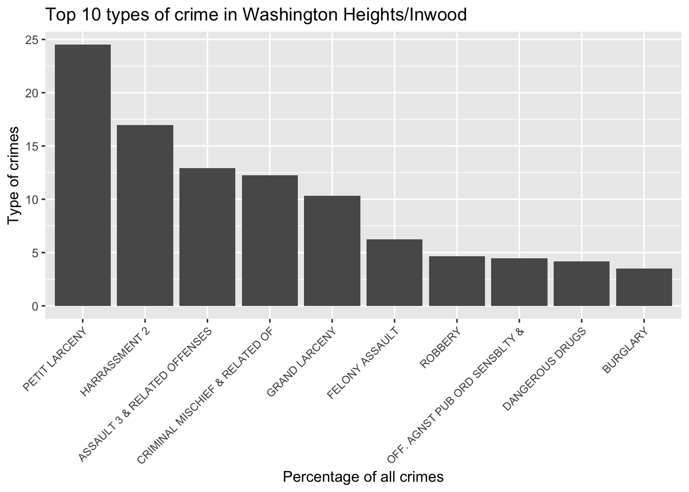
Rent & Crime Rate
Is there an association between rent and crime rate?
ses_df |> group_by(neighborhood) |>
summarise(avg_rent_0_1beds = mean(gross_rent_0_1beds),
avg_rent_2_3beds = mean(gross_rent_2_3beds)
, avg_crime_rate = mean(crime_rate, na.rm = TRUE)) |>
ggplot(aes(x = avg_crime_rate)) +
geom_point(aes(y = avg_rent_0_1beds, color = "Average Rent 0-1 Beds")) +
geom_point(aes(y = avg_rent_2_3beds, color = "Average Rent 2-3 Beds")) +
geom_smooth(aes(y = avg_rent_0_1beds), method = "lm", se = TRUE, color = "red") +
geom_smooth(aes(y = avg_rent_2_3beds), method = "lm", se = TRUE, color = "blue") +
scale_color_manual(values = c("Average Rent 0-1 Beds" = "red", "Average Rent 2-3 Beds" = "blue")) +
labs(title = "Point Plot of average rent against average crime rate",
x = "Crime rate",
y = "Average rent ($)") 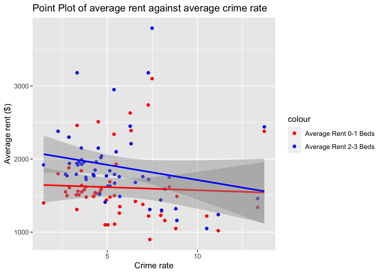
There appears to be no obvious association between rent and crime rate.
References
- Golub, Andrew, Bruce D. Johnson, and Eloise Dunlap. 2006. “Smoking Marijuana in Public: The Spatial and Policy Shift in New York City Arrests, 1992-2003.” Harm Reduction Journal 3 (August): 22.
- NYPD (2023, June 16). NYPD Complaint Data Historic: NYC Open Data. Link
- CoreData.nyc. Subsidized Housing Database. NYU Furman Center’s CoreData.nyc. Link
- Bureau, U. C. (2022, November 29). 2020 census. Census.gov. Link
- Department of City Planning (DCP) (2013, Jan 29). NYC Open Data. Link